Audio Equalizer – A Perspective on Digital Signal Processing

Digital Signal Processing plays a key role in today’s world, where television, sound systems, cameras etc are turning towards digital methods. Many signal processing such applications involve amplifying or attenuating only a small portion of a signal’s frequency spectrum, while leaving the remainder of the spectrum unaffected and one of such applications is a digital audio equalizer.

This effect is commonly obtained by using a digital filter that has poles or zeroes at specified center frequencies. Digital filter having a pole at a specified center frequency is called ‘resonant filter’ which enhances a specified frequency in the spectrum, while the filter having zero at a specified frequency is called ‘notch filter’ which attenuates a specified frequency in the spectrum of the input signal and leaves the rest of the spectrum unaffected.

In digital audio equalization, any desired frequency response can be obtained by cascading such filters with different center frequencies, where each cascaded system contains a pair of zeroes and conjugate poles.

By cascading a resonant and a notch filter an order system can be generated. If ‘r’ and ‘R’ are distances of zero and pole from the origin in unit circle and they are located at center frequency ω₀, transfer function of the system is given by,

Where,

In the transfer function H(z), zeroes are located at

  and poles are located at  Here complex conjugates of zeroes and poles are considered to get real filter coefficients.

Figure: 1

There are three possibilities to choose the values of ‘r’ and ‘R’ which are mentioned below.

1. If r < R, pole dominates and second order system H(z) works as a resonant filter at center frequency ω₀.
2. If r > R, zero dominates and second order system H(z) works as a notch filter at center frequency ω₀.
3. In this case, r > R or r <  R that means pole and zero are very close to each other at center frequency ω₀. If r > R, we get a notch at a center frequency ω₀ while if r <  R then we get a sharp peak at center frequency ω₀ and frequencies away from the ω₀ remains unchanged as shown in figure 1.

The third case is very important for the applications because frequencies other than ω₀ remains flat and we can easily get notch or resonator by small amount of change in the values of ‘r’ or ‘R’. This second order system is used in audio equalizer to enhance or attenuate particular frequency easily.

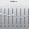
In the application of audio equalizer, more than one frequencies need to be controlled. An example of equalizer is shown in figure 2, where frequencies starting from 32 Hz to 16 KHz are mentioned at specific intervals and magnitude of each frequency can be modified up to 12 dB.

 Figure: 2

To implement transfer function of audio equalizer such second order filters are cascaded. Zeros & poles of every second order filter are located at different center frequencies which are 32 Hz, 64 Hz, 125 Hz, 16 KHz as shown in figure 2 and sampling frequency of 64 KHz is used as per Nyquist sampling theorem.

We are using 10 different frequencies in equalizer, so 10 second order filters are cascaded to implement transfer function of an equivalent system. As each cascaded filter is second order, equalizer system becomes of order 20.

If N is the no. of 2^nd order filter cascaded, transfer function of equalizer is given by,

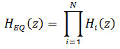
Where H_i(z) system is given by,

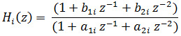
Where,

Figure: 3

Audio equalizer is implemented using MATLAB and simulation result of equalizer’s frequency spectrum is shown in figure 3. it shows that all mentioned frequencies are enhanced or attenuated as per the details shown in figure 2.

In the equalizer, each frequency has different values of ‘r’ and ‘R’ depending on its attenuation or amplification.  So we can easily enhance or attenuate any of given frequencies by just changing its value of ‘r’ or ‘R’.